T-tests are a fundamental statistical tool used in various fields, including public health, to compare the means of two groups. Essentially, a T-test helps determine whether the observed differences in data sets (such as rates of a disease, responses to a treatment, or other health indicators) are statistically significant or likely due to chance. This test is vital in research and data analysis, as it provides a scientific basis for drawing conclusions about populations based on sample data. Whether it’s comparing the effectiveness of different treatments, understanding health outcomes across different demographics, or analyzing behavioral health interventions, T-tests offer a reliable method for making informed, evidence-based decisions in public health and beyond. Here, we’ll take a look at how to run a T-Test in R.

Background: Understanding T-Tests

Before we look at how to run T-Tests in R, it’s worth understanding what we’re actually doing. As mentioned above, a T-Test is at its core, a comparison between two groups to see if they are different from each other in a way that cannot be explained by simple chance.

Types of T-Tests

There are 4 main groups of T-Tests that one may need to choose from when testing a hypothesis. These are:

• Sample Dependent:
  • Independent Samples T-Test (Two-Sample T-Test):
    • Purpose: Compares the means of two independent or unrelated groups.
    • Example: Comparing the blood pressure of patients who received two different treatments.
  • Paired Samples T-Test (Dependent Samples T-Test):
    • Purpose: Compares the means of the same group or matched pairs at two different times or under two different conditions.
    • Example: Measuring students’ test scores before and after a training program to assess its effectiveness.
  • One-Sample T-Test:
    • Purpose: Compares the mean of a single group against a known mean (or a theoretical value like zero).
    • Example: Testing if the average height of a group of individuals differs from a specific value, like the national average.
• Tail Dependent:
  • One-Tailed T-Test:
    • Purpose: Tests for the possibility of the relationship in one specific direction.
    • Example: Testing if a new drug increases recovery rates compared to the existing standard (only looking for an increase, not a decrease).
  • Two-Tailed T-Test:
    • Purpose: Tests for the possibility of the relationship in either direction, without specifying which direction is expected.
    • Example: Testing if a new drug changes recovery rates (either increase or decrease) compared to the existing standard.
• Assumed Variance:
  • Equal Variance T-Test (Pooled Variance T-Test):
    • Purpose: Used when the variances of the two groups are assumed to be equal.
    • Example: Comparing the test scores of students from two classes where the variation in scores is similar in both classes.
  • Unequal Variance T-Test (Welch’s T-Test):
    • Purpose: Used when the variances of the two groups are not assumed to be equal.
    • Example: Comparing the test scores of students from two schools where one school shows much greater variation in scores than the other.
• Assumption of Non-Normal Distribution:
  • Robust T-Tests:
    • Purpose: Used when data do not meet the assumptions of normality. These are variations of the T-test that are less sensitive to non-normal distributions.
    • Example: Comparing means from data with outliers or skewed distribution.

This is a very broad overview of each category, and we’ll cover more in our Epi Explained series entry on T-Tests. For now, we’ll focus on perhaps the broadest and most generally applicable T-Test for our tutorial, the 2 tailed T-Test. Let’s get started.

Mathematical Underpinnings

In terms of the underlying math for T-Tests, it’s not quite as easy as our previous topics of Odds Ratio and Relative Risk, and can even seem a bit intimidating, but let’s break it down a little bit.

[math] t = \frac{\bar{X}_1 – \bar{X}_2}{\sqrt{s^2 \left(\frac{1}{n_1} + \frac{1}{n_2}\right)}} [/math]
The above formula is for what is called the T-Statistic. Its components are interpreted as:

• [math] \bar{X}_1[/math] : The mean of Group 1
• [math] \bar{X}_2[/math] : The mean of Group 2
• [math] s^2[/math] : The Pooled Variance, which requires another formula we’ll cover below.
• [math] \frac{1}{n_1} [/math]: 1/ the sample size of Group 1.
• [math] \frac{1}{n_2} [/math]: 1/ the sample size of Group 2.

Now for the Pooled Variance. In short, Pooled variance is a weighted average of the variances of the two above samples. As a reminder, variance is the squared difference between each value of a group and the mean of said group, finally divided by the number of the group – 1. the formula for Pooled Variance is:

[math] s_p^2 = \frac{(n_1 – 1) \times s_1^2 + (n_2 – 1) \times s_2^2}{n_1 + n_2 – 2} [/math]

Where:

• [math]s_p^2 [/math] is the pooled variance.
• [math]n_1[/math] is the sample size for Group 1.
• [math]n_2[/math]is the sample size for Group 2.
• [math]s_1^2[/math] is the variance for Group 1.
• [math]s_2^2[/math] is the variance for Group 2.

It might be worth noting that the denominator, [math]{n_1 + n_2 – 2}[/math] is the calculation for the Degrees of Freedom (DF), which will be a critical calculation in many other statistical operations.

After calculating through these equations, the final step is to reference a T-Distribution table with your Degrees of Freedom and the level of significance (p value) you wish to use, and see if the value is larger than the referenced table value. If the equation value is more than the reference value, then your results could be considered significant. Otherwise, any differences are likely to be due to chance.

With the underlying math out of the way, let’s look at how we can do a T-Test in R, using real world data.

Calculating A T-Test in R

As usual, if you’d like to follow along with full code write-up and data, please go to Cody’s Github and download the T-Tests folder.

Step 1: Library set up

For our tutorial, we’re only going to need the base R packages, and tidyverse which is mostly used for our data cleaning. We can install and load this library using the following:

Step 2: Collect and Format Data

Now, we can take a look at our data. For this tutorial, we’ll be borrowing some data from the Northern Irish Statistics and Research Agency (NISRA), particularly their data around the number of suicides in North and South Belfast Assembly Areas from 1997 to 2018. We can have as a null hypothesis that there is no difference in suicide rates between North and South Belfast.  I’ve pulled a CSV which has two rows (one for North Belfast, another for South), and the columns are
Assembly.Area and then every other column is a year with an X in front of it. This closely resembles data you’re likely to experience in the field, as it’s a mess and not formatted how we’d like. Let’s quickly read in the file, and then look into all of the column names except the first, and remove  any X’s in front of the years.

Now that our data is cleaner, we can format it a bit. While there are perhaps more efficient ways to go about it, I think this makes for a good time to look at long and wide dataframe transformations. As our data is now, it’d be very hard to fit into a T-Test calculation, as we cannot easily iterate across columns to collect the values (counts per year) we need for our groups (location). It could be said to be very wide. Let’s transform it to a longer format.

Here, we’ve taken our dataframe and “piped” %>% it so we can do multiple transformations on it. We then used the pivot_longer function to rearrange our dataframe, by making sure our Assembly Area keeps as a column, but then making two new columns, Year and Count. Year is essentially taking the names of the original dataframe columns and putting them as a row value, and then taking their value and saving it as Count.

This does make the data a bit cleaner, but ideally we’ll have to make this a bit wider by have a separate column for each of our location groups, and a reference column to our Year. This will look remarkably similar to above.

Now that our data is properly formatted, let’s get to testing.

T-Test in R: The Easy Way

The easiest way to run a T-Test in R, now that we have our data formatted, is just calling the T-Test function against our groups, like so:

When we look at t_test_resultin our Console, we can see that there’s a very significant difference between the two locations.

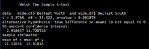
And there we have it.

T-Test in R: The Hard Way

Say for whatever reason, you don’t quite trust the above function to do all the hard work for you and want to handle this all manually. Then, we can use the code below which is fairly self-explanatory (given the above mathematical discussion). There isn’t too much to delve into as it’s mostly simple calculations that are absent any complex functions.

Conclusion

Here, we took a look at what T-Tests are, the math underneath the term, and even how to use them in R to answer a question about suicide rates in Northern Ireland.

Humanities Moment

This tutorials painting is Bangor, Belfast Lough by James Arther O’Conner (Irish, 1792-1841). A landscape painter with a rather incredible reputation, O’Connor exhibited his work at the Royal Academy in London, England in 1822. His works often feature a notable sense of depth and atmosphere, capturing the moody and dramatic skies, lush countryside, and the serene beauty of rivers and lakes. He had a talent for rendering light and shadow, which added a dynamic and often poignant quality to his landscapes.