
Introduction
Odds Ratio (OR) calculations are a cornerstone in public health research, providing insights into the strength of association between an exposure and an outcome. In this ThuRsday Tutorial, we’ll explore how what an Odds Ratio is, as well as how to calculate it in R.
Understanding Odds Ratio
Odds Ratio (OR) is a measure used in epidemiology to compare the odds of an event occurring in one group to the odds of it occurring in another group. This is especially useful in case-control studies where you’re comparing the odds of exposure in cases (those with the disease or outcome of interest) to the odds of exposure in controls (those without the disease).
Odds as a Concept
Before diving into odds ratios, it’s important to understand what “odds” are. In a health context, odds are a way of representing the likelihood of an event happening. If the probability of an event happening is P, the odds are calculated as:
[math]{\text{Odds} = \frac{P}{1 – P}}[/math]
Simply put, this equation reads as “Odds can be calculated as the probability of an event occurring [math]{(P)}[/math], divided by the probability of the event not occurring [math]{(1 – P)}[/math]”.
Calculating the Odds Ratio
Now, consider a case-control study with the following data:
- : Number of cases (people with the disease) who were exposed to a certain risk factor.
- : Number of controls (people without the disease) who were exposed to the same risk factor.
- : Number of cases who were not exposed to the risk factor.
- : Number of controls who were not exposed to the risk factor.
The odds of exposure among the cases is [math]{A/C}[/math], and the odds of exposure among the controls is [math]{B/D}[/math]. The odds ratio is calculated as:
[math]{\text{Odds Ratio (OR)} = \frac{\text{Odds of exposure in cases}}{\text{Odds of exposure in controls}} = \frac{A/C}{B/D} = \frac{A \times D}{B \times C}}
[/math]
Interpretation of the Odds Ratio
- OR = 1: This suggests there is no association between the exposure and the outcome.
- OR > 1: This indicates a positive association, meaning the exposure might increase the odds of the outcome.
- OR < 1: This implies a negative association, suggesting the exposure might decrease the odds of the outcome.
Limitations
It’s important to remember that odds ratios can sometimes overestimate the risk, especially if the outcome is common. Also, they do not necessarily imply causation.
For more explanation on the underlying mathematics and mechanics of Odds Ratios, please check out our Epi Explained series! For now, let’s get on with the calculation of Odds Ratios in R.
Odds Ratio in R: Smoking and Cancer
For our tutorial, we’ll run with a fairly simple assignment. If you’d like to follow along with this tutorial, download the folder for Odds Ratio on Cody’s Github. Imagine that you’ve been handed a dataset by a senior epidemiologist, where you need to figure out if smokers have a higher odds of presenting with two cancer diagnoses, either malignant mast cell neoplasms (C96.29) or malignant neoplasm of unspecified part of unspecified bronchus or lung (C34.90).
Preliminaries: Installing and Loading Required R Packages
Before diving into the analysis, ensure you have the necessary libraries. Install and load ‘dplyr’ for data manipulation and ‘epiR’ for epidemiological analysis in R, as shown below:
Importing and Preparing the Dataset
Now we can import our sample data, saved as “smoking_survey.csv”. To help better simulate real world data, this spreadsheet isn’t quite the format we’d need for our analysis, so we’ll need to do some cleaning. For now, we can call the base R function read.csv() to put our data into a dataframe.
Now we can inspect our data and see there’s 3500 rows of 5 variables. X appears to be just a counter, smoking_status seems to be filled with either “smoker” or “non-smoker”, age is the age of the person, diagnosis_codes appears to be a list per person of various ICD-10 codes, and then we have a zipcodes field.
Data Transformation for Analysis
Next, we select the relevant variables: smoking_status and lung_cancer. We can then create a function to mark ‘yes’ for lung cancer diagnosis based on specific codes and ‘no’ otherwise. This next bit of code might be tricky for new users, so let’s break it down.
Here, we did the aforementioned selection of columns we want to deal with using dplyr::select(), telling it to reassign our dataframe to just these values. Our next step is to create what is called a function. Functions are pieces of code that can be run multiple times or be used to organize certain operations in a way that results in cleaner code. As a rule, if you’re doing something more than twice, or if it’s something that might require some alterations in future (say, needing to add a new diagnosis to search for), a function can be the way to go. What we are doing is creating a function called has_lung_cancer which takes in the argument codes.
Next, it creates an if statement, where if there is a match to the condition, the code does one operation, and if it doesn’t, another takes place, or the operation is passed over. In this case, we’re using the grepl operation to scan through our column of choice to look for first “C34.90” and then “C96.29”. If it matches in either case ( || is an “OR” operator) then we get a value of “yes” returned, otherwise “no”. Keep in mind that this match can be at any point in our column for each row, so it can start with the code, end with the code, or have it somewhere in the middle and it won’t matter as it’s just looking for a match and ignoring everything else through what are called Regular Expressions (ReGex), which will be a later topic.
Applying the Diagnosis Function
Now we can actually apply this new function to our dataset, and have something that’s much easier to work with. Here, what we’ll do is create a new column in smoking_survey called lung_cancer. We’ll then fill this field by taking the smoking_survey dataframe, and going down row-wise (the 1 indicates we’re going down rows, where 2 would indicate going across columns), and apply a function that calls the has_lung_cancer function down the diagnosis_codes column.
From there, we just do another selection operation to get rid of our diagnosis codes, and then turn our column values into a data type called factors . In short, factors are basically categories that make things easier to arrange, and we then tell R within our factor call to make 2 specific categories for each column, and how they should be arranged for future use.
Creating a Contingency Table
A contingency table lays the foundation for calculating Odds Ratio. We can create a table with smoking_status and lung_cancer to visualize the distribution using the table() table. We can see that there’s very obviously a difference in counts, especially accounting for the uneven sample sizes of smokers and non-smokers. Now that we have our contingency table, we can calculate our Odds Ratio manually. This is a rather simple operation as all we need to do is take our smokers groups and dvide them by our non-smokers groups (our with event and without events). the [Y,X] after our table name basically points out the position, where Y is our Column and X is our row.
And there we have it, how to create our Odds Ratio manually, arriving at a value of 5.77, which indicates smoking does increase the likelihood of getting cancer profoundly. However, there’s another process that can provide us these values as well as many other statistics to examine if that value is significant.
Using the epiR Package for Odds Ratio Calculation
The ‘epiR’ package simplifies this process. We use the epi.2by2 function for a more comprehensive analysis, including confidence intervals. All we need to do is set our method to cohort count, set a confidence level, and get a quick format to return the results in.
Now we can check the results in our terminal: 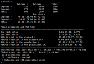
Conclusion
Here, we’ve learned what Odds Ratios are, how to calculate them both by hand and in R, and how to leverage both functions and the EpiR library to make our analysis easier and more comprehensive.
Humanities Moment
The featured image of this article is Small River House (1913) by Amadeo de Souza-Cardoso (Portuguese, 1887 – 1918). Initially influenced by impressionism and then by cubism and futurism, this Portuguese painter became a pioneer of modern art around 1910, known for his aggressive, vivid style that often verged on abstractionism or dadaism. His participation in the 1913 Armory Show in the U.S. marked the beginning of a highly experimental career, though he didn’t gain wide public recognition until the 1950’s.