
In our last article, we covered how to handle reading in CSV and XLSX data into R and some basic cleaning of said data. Today, we’re going to go from properly reading in the data, to making data products and figuring out what it can tell us. Let’s take a look at how to do Exploratory Data Analysis in R. To follow along in this Exploratory Data Analysis, feel free to pull the data and code from our GitHub.
Data Background
Before we get into the analysis portion of the article, let’s first take a key step in any exploratory data analysis and do some background work on the table we’re working with.
As you may recall, we are using the Northern Irish Statistical and Research Agency (NISRA)’s collection of reported suicide records from 1970 until 2018. For today’s exercise, we’ll actually be only looking at one table we made in our last article, Table 3, or the recorded rate per 100,000 by Sex. This table has only a couple of main variables that we need to pay attention to. These are the Registration Year, the counts of Male and Female presumed cases, and the total count of presumed cases per Registration Year.
While most are self-explanatory, the term Registration Year may seem a bit ambiguous. Simply put, this was the year in which the case was registered with the Coroner, which means, as you might expect, there were often delays from the event to the registration. In the original Excel workbook released by NISRA, table 13 shows the median lag between event and registration from 2001-2018. Though we cannot be sure, we can assume with some level of safety that those dates before 2001 had at least as much as the median delay, which means any analysis we perform has to have a caveat that the particular count of any one year might actually be a delayed effect of a particularly bad year previous.
On the topic of data constraints, we are also limited by the ability to define what suicide is to any level of certainty. Certainly, back when I worked primarily with suicide and overdose data, this was always a problem. We cannot be in someone’s mind post-event, and so our estimates will always be imperfect to some degree, so looking at general trends is perhaps most beneficial. For NISRA’s standards, they are counting a case using the following definition:
In the UK, in considering suicide events it is conventional to include cases where the cause of death is classified as either ‘Suicide and self-inflicted injury’ or ‘Undetermined injury’. The ICD codes used for ‘Suicide and self-inflicted injury’ are X60-X84 and Y87.0 (ICD9 E950-E959), and the ICD codes used for ‘Undetermined injury’ are Y10-Y34 and Y87.2 (ICD9 E980-E989).
-NISRA
This can be seen as a slightly conservative approach, though by no means an incorrect one, and may one day be a topic unto itself. But for now, that’s enough background on what the data is and the limitations therein, let’s get to seeing what this data can actually tell us.
Exploratory Data Analysis – Data Read-In and Basic Statistics
Since we will be dealing primarily with numerical data in this exercise, our first tasks are going to be quite easy. Step one, of course, is reading in our data just like we did last time. We’ll save it as a DataFrame called Rate_Per_100k, just to make sure we remember what we’re looking at should we need a quick break.
#Load in packages for later use
pacman::p_load(
  tidyr,
  ggplot2,
  plotly
)
# Read in File
Rate_Per_100k <- read.csv("table3.csv")
Now upon inspection, we’re seeing one extra variable called X that we really don’t need.
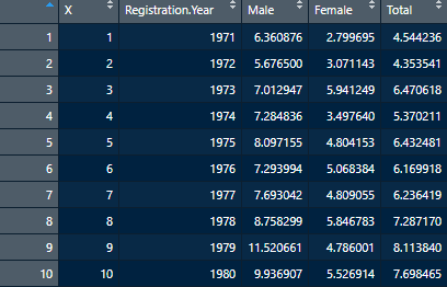
That’s not ideal, so we’ll clean that up really quickly using a method similar to what we’ve done in the past. Just instead of deleting a row, we’ll take out a column using:
Rate_Per_100k <- Rate_Per_100k[,-1]Recall that calling a DataFrame in this way is telling R to retain all rows (empty before the comma), and all but the first column. Now that we’ve got that cleaned up, we can go about calculating some basic statistics. For this exercise, we’ll calculate the Mean, Median, Standard Deviation, Variance, Minimum value and Maximum values for the Male, Female and Total columns. We could repeat several commands in the script a few times, or we could build what’s called a function and make life a bit easier for ourselves.
# We want to create 3 seperate DataFrames for Male, Female, and Total. Since a lot will be repetition, let's use something called a function.

Core_Stats <- function(DataFrame, colname){

  #for these calculations, we need to pull from the list of values, transform them into a numeric vector, then run the calculations
  Avg <- mean(as.numeric(unlist(DataFrame[colname])))
  Median <- median(as.numeric(unlist(DataFrame[colname])))
  StD <- sd(as.numeric(unlist(DataFrame[colname])))
  Variance <- var(as.numeric(unlist(DataFrame[colname])))
  Min <- min(DataFrame[colname])
  Max <- max(DataFrame[colname])
  Category <- colname

  Core_Stat_Block <- data.frame(Category,Min, Max, Avg, Median, StD, Variance)
  return(Core_Stat_Block)
}
Here, we are creating a function we can use multiple times called Core_Stats. For Core_Stats, we’ll feed in the name of a DataFrame (in this case, Rate_Per_100k), as well as a column name (“Male”, “Female”, or “Total”). From there, we take the fed in DataFrame and create variables for the above-listed statistics. To make sure everything is correctly computed, we take the original DataFrame Column, which is considered a list, and then unlist it to a vector that is then interpreted as a vector of numbers. If this doesn’t make sense immediately, that’s okay. We’ll cover data types in a future article, but for now, know the general rule that math operations don’t like working with lists, so when we see them, we need to transform them. For reference, min() and max() don’t quite require this reworking as it’s acting more like a search function. Lastly, we grab the colname so we can use it as a label, combine all the variables into a DataFrame and return it out of the function.
Since the function is now done, let’s test it out by creating 3 DataFrames, one per column of interest, combining them, and doing away with the intermediate DataFrames.
Female_CS <- Core_Stats(Rate_Per_100k, "Female")
Male_CS <- Core_Stats(Rate_Per_100k, "Male")
Total_CS <- Core_Stats(Rate_Per_100k, "Total")

#Now row bind (rbind) them to one DataFrame. Can use for tables later
Stats_DataFrame <- rbind(Female_CS, Male_CS, Total_CS)

#and remove unneeded DFs
rm(Female_CS, Male_CS, Total_CS)
This creates a DataFrame which can then be turned into tables, which again we’ll cover in another article. An example of such a table is below:
| Category | Min | Max | Avg | Median | StD | Variance |
|---|---|---|---|---|---|---|
| Female | 2.799695 | 8.025987 | 5.417896 | 5.217563 | 1.597635 | 2.552437 |
| Male | 5.676500 | 27.137226 | 15.774356 | 14.328779 | 6.360067 | 40.450452 |
| Total | 4.353541 | 17.394765 | 10.482895 | 9.197285 | 3.718632 | 13.828223 |
The table does give us some quick and useful insights. Namely, every single statistical measure points to those assigned Male at birth had a higher rate of suicide cases per 100,000 individuals and much more variability in case numbers, despite Male and Female being somewhat even in the country (49% and 51% respectively) and the population being above 1.5 million since 1970 and currently reaching nearly 2 million people. But what this does not tell us easily is if this initial analysis is due to a spike, or is a common trend in time. Plus, it’s a touch hard to read, so let’s look at making some visuals.
Exploratory Data Analysis – Creating Graphs
So before we can make some graphs, we need to do a tiny bit of data cleaning and make our data long as opposed to wide, which was covered in our previous article. In short, we turn the Male, Female and Total columns into one column we name ASAB (Assigned Sex at Birth), and use the Count field to keep track of the number of cases per ASAB per Registration Year.
Rate_Per_100k <- Rate_Per_100k %>%
  tidyr::pivot_longer(cols = c("Male", "Female", "Total"))

#rename columns
colnames(Rate_Per_100k) <- c("RegYear", "ASAB", "Count")
One of the biggest reasons to use R, period, is how very easy it is to create graphs in R and customize every little detail. As such, it’s also a great advantage when doing XDA (Exploratory Data Analysis), as you can really dig into the data quickly, and go from idea to image easily. To prove this, let’s make a quick box plot using ggplot2, one of the best graphics libraries for R.
#Create Boxplot
BoxPlot <- ggplot2::ggplot(data = Rate_Per_100k) +
  geom_boxplot(mapping = aes(x = ASAB, y = Count)) +
  labs(title = "Suicides per 100,000, 1970-2018 by Assigned Sex at Birth",
         subtitle = "Median based Box Plot",
         caption = "Data source: NISRA.gov.uk")
In the above code, we call ggplot2’s ggplot to draw a graph using our Rate_Per_100k DataFrame. We then use the plus symbol to tie in another graphical function to tell ggplot2 we want a box plot, with the X to be Sex, and Y to be the Count of cases. The labs, as you may have guessed, are labels to be used. This produces the following:
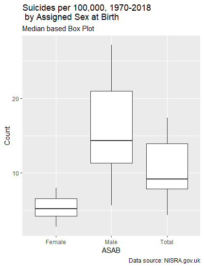
This essentially covers the same information as the table above did, but does it in a way one can understand at a glance. Now let’s look at how to do some timeseries-based analysis using an interactive library, plotly.
Plotly is another graphing library that is formatted similarly to ggplot2, but provides the advantage that the images are not static, so they can provide more information and even allow for some filtering. The code for our next graph is as follows:
#Create interactive graph using Plotly
plotly::plot_ly(data = Rate_Per_100k, x = ~RegYear, y = ~Count, color = ~ASAB) %>%
  add_lines()  %>%
  layout( title = "Interactive Timeseries: Suicides by Sex and Year, 1970-2018" , xaxis = list(title = 'Registration Year'),yaxis = list(title = 'Rate per 100k'))
Here, we are taking the plot_ly function, similar to ggplot2’s ggplot function, and telling it we want to use our DataFrame, and to iterate down values using “~” in front of column names. We’re then piping in the add_lines() function to put lines between the default scatter plot, and then piping again to get our titles in. The end result for us is something somewhat simple, but given that it’s 4 lines of code, mighty impressive as well.
As we can see, there’s a general upward trajectory in Males, and it’s mostly flat for Female cases, but there is a remarkable spike in 2006. This may lead us to further look at the years 2004-2006 to see what may have changed.
Exploratory Data Analysis – Findings and Conclusion
Given our table and graphs, we can say that Suicide Cases which are registered are more likely to be from Males. They also have less stable case rates overall, and we may want to look at the mid-2000s and what may have happened during that time period to greatly increase the case counts before they stabilized in the ensuing decades. For Female cases, we may want to look at the early 1970s, early 1980s, and mid-2000’s to also see what may be contributing factors.
As you may have guessed, Exploratory Data Analysis is, more than anything, a starting point. We don’t have answers, and we have no promise of answers, but we do have some initial findings which could lead us to greater insights. We also know around what times we should look for events or factors, down from 5 decades to maybe 10 if we’re being particularly thorough for any one demographic. I would in particular also look for different ways the data has been chopped up to see if more information could be gained.
In this article, we covered what an Exploratory Data Analysis looks like for primarily Numeric data, and how to present some basic findings. If you’d like to test it out yourself, please visit our GitHub to download the code and data. In the future, we will be looking at how to do XDA on text data, starting a whole series on Natural Language Processing.