
If you haven’t gotten the email, you will soon. “Hey there, I was wondering if you could tackle an analysis of this data? Thanks!” The tone’s cheery, and surely this shouldn’t take too long, right? How much data can be emailed in an Excel file? And they’re all tables, computers love tables, right? Well, not always. But don’t worry! In this article, we’re going to tackle how to read Excel files into R, both the common CSV files and the more complex XLSX workbooks. Be sure that if you haven’t yet, download R and RStudio. Let’s get into it.
Read Excel Files in R
Hate it or love it, Excel has been a mainstay of both Public Health for quite a long time. It’s become such an “old reliable” in our field that it’s been at the heart of several major incidents, such as when Public Health England relied on Excel (admittedly, an archaic file format for Excel called XLS) a bit too much and lost 16,000 COVID swab test results. Incidents aside though, when working at any level in the field, you’re sure to get emailed excel tables that look great, at least originally.
The problem lies in what is easy for computers to read, versus what is easy for humans to read. You see, we like titles up at the top telling us what the point of a table is. We like formatted tables that combine and chop up groups, ages, whatever, so we can note any strange patterns or comparisons. And by whatever Almighty you believe in, do we ever love having more than 1 observation per row of a table. We often use these factors to decide how to build tables for each other, but what do computers like? Let’s kick on RStudio and see first what it sees from a formatted table, and then what we need to do to fix it.
Starting out, we’re going to grab an Excel workbook from the Northern Ireland Statistics and Research Agency. Specifically, we’re going to be pulling their death counts from 1970-2018 which are presumed to be suicides. We will be looking to use this data in other analyses in future articles, and thus making sure we read the data correctly is crucial. If you’d like, you can pull these files from the NISRA website itself, or via my Github, in the DataSets section. Upon opening up the file, you’ll see that there is quite a selection of tables that we could pick from, but for today’s exercise, I’m going with Table 2 and Table 3.
For both tables, we’ll need to do a bit of the same process, but let’s go through the operations on each table individually as practice. Let’s begin by just looking at what Table 3 looks like in Excel, not in R quite yet.
Read Excel Files in R – Easy File
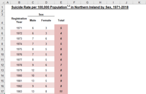
Okay, so that doesn’t look too bad. We have a clear title, labels for each column, and even a nifty categorization of Male and Female as Sex. Whoever designed this did a great job in terms of readability. Now that we know what it’s supposed to look like, let’s get some code going.
Before we can read in the excel file into our R environment, we need to load the necessary libraries. You can think of libraries as packages of prebuilt tools you can use in your programming to make life significantly easier. Typically, if you need to install a singular package, one can use the following:
install.packages("pacman")
In this case, we’re looking to install the package pacman, from the Comprehensive R Archive Network, or CRAN. Pacman is incredibly useful as it has a function called “p_load”, which checks to see if you have the packages you need installed. If they are, then it simply loads those packages into the environment you’re working in. If not, it will install, then load those packages, which is great for sharing code. In general, you want to keep your install.packages() commands outside of your main script (use the console at the bottom), while “p_load” can be used in the script, as seen below:
pacman::p_load(
  readxl
)
Here, we’re telling R that we want to dig into the pacman package, find the “p_load” function, and then use it to load in readxl, which is a library that’s used to, as you might guess, better read excel files. We can now use read excel to bring in that xlsx file into the R environment and take a look at how R sees the excel file. Below, what we’ll do is name a variable (basically a data storage container) Table_3_DataFrame, and we’ll define its contents as the result of reading an xlsx sheet, namely the one found at the path name, and then the specific sheet called “Table 3”. Do keep in mind that if your R code is not saved to the same folder as your excel document, you’ll need to lengthen your path to find it. For instance, it could be “C:/User/Sheets/” and then the file name.
Table_3_DataFrame <- readxl::read_xlsx(path = "00_Suicide_2018_NOT_CLEANED.xlsx", sheet = "Table 3")
Good, now we can click on the table icon next to the newly named DataFrame to see how it looks.
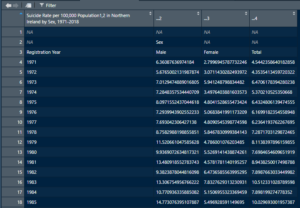
That isn’t great. But that’s alright, let’s list off some of the issues we see off the top. So for the column names, it did catch the title of the whole table, and did bring in the right number of columns. We also have all the data after the table titles looking just fine, and it looks like row 3 could really be our column header without any real editing. We have a plan forward, let’s just cut off everything above row 3.
To do this, we really need to only adjust the read in command we just did to something a touch more specific.
readxl::read_xlsx(path = "00_Suicide_2018_NOT_CLEANED.xlsx", range ="Table 3!B4:E52")Now, instead of using just sheet, we’re actually using a range argument instead, which takes in the table, then an exclamation point to denote where that title ends, and then the upper left, and lowest right cells that contain data. As a general piece of advice, you can find a lot of information by using the following in the console to find out more about certain functions:
?Package::FunctionInPackageThis will open up a small page in Rstudio that will let you know all the fun things you can do with any specific function, and is probably the most useful command you’ll use outside of bringing packages in. Anyways, back to the task at hand, with this new parameter of range, let’s see how we did.
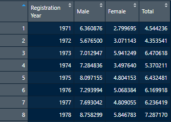
Perfect, we have column headers where they need to be, and the data is clean and easy to read. We can now save this as a CSV file if we so wish, and move on to the next table.
write.csv(Table_3_DataFrame, file = "Table3.csv")As with our read-in, we can also change where the file is saved with a path before the “Table3.csv” file name. Now for a real challenge.
Read Excel Files in R – Challenge File
Now that we have a nice warmup done, let’s take a look at a much more challenging table, Table 2, shown here:
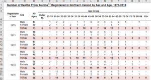
So now we have null values represented by “-“, zeroes, some of the formatting issues we saw earlier, and a lot more column entries that would be hard to work with in R, as R is more oriented towards going down rows and not across columns for many functions. As before, let’s take a look at what happens when we read in the Excel data into R.
pacman::p_load(
readxl,
zoo, # We'll need this and tidyr later for some special functions
tidyr
)

Table_2_DataFrame <- readxl::read_xlsx(path =  "00_Suicide_2018_NOT_CLEANED.xlsx", sheet = "Table 2!B3:T151")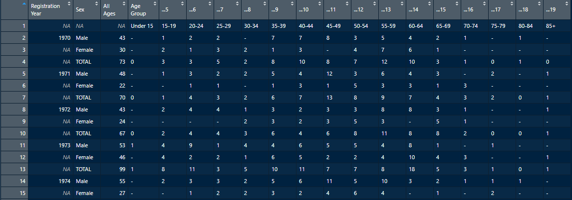
It doesn’t get much worse than that. We have all the problems we already saw off the bat in the excel sheet, and misaligned columns, plus a bunch of rows without years. This would be useless for analysis, so let’s break down what we need to do into a few steps:
- Set the columns to have names in their proper places.
- Find a way to get those entries with missing years their proper year assigned
- Pivot the data from a wide format as it currently is, to a long format so that each age group gets its own row as opposed to its own column.
- Reformat any labels as needed.
Step 1, we can perform a simple enough operation of just cutting off that first row entirely that has mostly numeric-based titles and then renaming the columns by age group. You might wonder why we don’t just push the numeric-based titles up, and mostly it’s to ensure that there aren’t weird interpretation errors in R. As a rule, you don’t want variables to start with a number. So, we can subtract the row in question by calling a DataFrame to assign its values to itself, except for that first row, as seen here:
Table_2_DataFrame <- Table_2_DataFrame[-1,]
In this case, the square brackets tell R you want to do something inside a variable, and within DataFrames you can (usually) treat the square brackets as holding two values in format X,Y. In this case, we want all but the first X (row), and we want all columns, so we put nothing there after a comma. Now that we’ve got that bit sorted, let’s handle renaming everything.
 colnames(Table_2_DataFrame) <- c("RegYear", "ASAB", "AllAges",
 "AgeGroup1", "AgeGroup2", "AgeGroup3", "AgeGroup4", "AgeGroup5","AgeGroup6",
 "AgeGroup7", "AgeGroup8","AgeGroup9", "AgeGroup10", "AgeGroup11", "AgeGroup12",
 "AgeGroup13", "AgeGroup14", "AgeGroup15", "AgeGroup16")
Now, this seems clunky, and you might be asking the great question of why we don’t just name the Age Groups as their respective numbers (i.e., 05-17). This is primarily because naming variables or column headers with numbers is seen as bad practice and can cause errors.
With that out of the way, we can now fill in those missing year values. This is an easy enough problem to logic out, we just take a look at the RegYear value, and if it’s empty, fill it in with the value that came before it. the zoo package is super handy for this sort of work.
Table_2_DataFrame$RegYear <- zoo::na.locf(zoo::na.locf(Table_2_DataFrame$RegYear),fromLast=TRUE)
Every year is filled in, so now it’s time for something a bit weird. As the table is now, it’s termed as “wide”, which is to say the observations are considered the years, and the different number of people in each age group is part of that observation. To make analytics easier, later on, we’re going to make it “long”, which is to say each year, and each age group will be its own observation.
Table_2_DataFrame <- Table_2_DataFrame %>%
tidyr::pivot_longer(cols = starts_with('AgeGroup'))
Since you’ve been paying attention to the code up to this point, you might think this looks very strange. Namely, what does “%>%” do in R? What is it, even? “%>%” is called a pipe, from the magrittr package, and what it does is for more complex function calls, or for multiple function calls using the same dataset, makes it so you needn’t retype anything. The %>% tells R “Take this data, and default to it being the object I want to do stuff on in future functions”. You can link multiple pipes together, and in one particular script I bore witness to a 100-line long piping operation. As a general rule, and as a personal plea, don’t do that. Once the piping is done, the function to make the DataFrame longer is told to make the columns that start with “AgeGroup” into a reference to our new rows. Keep in mind due to this operation, some column names changed.
Next, we can take out those pesky “-” values and replace them with R’s native Null value, NA. The reason we do this is to ensure that age value columns can be converted from a string value, which can’t be manipulated numerically, to a numeric column that can only contain null or numeric values.
Table_2_DataFrame$value[Table_2_DataFrame$value == "-"] <- NA
Almost done now. All that’s left is renaming the Age Groups, some column names, and turning Assigned Sex at Birth (ASAB) into a factor (category), and our counts of cases into a numeric column.To change the values of age groups, we’ll call the data frame, then look for the value “name”, which is what those AgeGroups ended up changing to. Then, we’ll tell R to look for values in that column that are equal to the value of that age group, and reassign the values. To change the columns, the names() function acts similarly.
 #replace AgeGroups
NI_DF["name"][NI_DF["name"] == "AgeGroup1"] <- "Under 15"
NI_DF["name"][NI_DF["name"] == "AgeGroup2"] <- "15-19"
NI_DF["name"][NI_DF["name"] == "AgeGroup3"] <- "20-24"
...
NI_DF["name"][NI_DF["name"] == "AgeGroup15"] <- "80-84"
NI_DF["name"][NI_DF["name"] == "AgeGroup16"] <- "85+"

#Or if you want a quicker way about it, try creating a list of the year groups and age groups and iterate down them.
#We'll cover that in a later article.

names(NI_DF)[names(NI_DF) == 'name'] <- 'AgeGroup'
names(NI_DF)[names(NI_DF) == 'AllAges'] <- 'AllAgesCounts'
names(NI_DF)[names(NI_DF) == 'value'] <- 'Counts'
NI_DF$ASAB <- as.factor(NI_DF$ASAB)
NI_DF$Counts <- as.numeric(NI_DF$Counts)
And there we have it, now we can save the results into a CSV file to use later. Speaking of CSVs, let’s cover how to quickly read CSV files into R.
Read CSV Data in R
Unlike what we’ve covered so far, reading in CSV files is remarkably straightforward. This is due to the fact that by definition, CSV files typically have very little room for formatting customization and thus R can usually be depended on to read in these files with no problem.
To practice, we’re just going to pull in a CSV we already made from the previous section. All you really need is “read.csv” from the Utils package which is bundled up in base R. So, instead of a few steps like we did above to get the data into a properly readable state, we just need the following one-liner:
Test_DF <- read.csv("Table3.csv")
And there you have it. As a note, I have seen a few people try just using “read.csv” without assigning it a variable, which R will allow you to do, it just isn’t terribly useful unless you are planning some very complex manipulations as the data comes in. Instead, defining a DataFrame variable as we did above is the norm.
This concludes our short article on how to read Excel files in R. In our next article, we’ll explore how we can go about performing some exploratory data analysis on a few of these files. As usual, if you’d like to try out some operations on the same data used in this article, or check out the full code solutions to what we did today, check out my personal Github, where I have a folder for each article written.